Butterflies are not only beautiful creatures but also important indicators of a healthy ecosystem. Identifying butterfly species can be a challenging task, even for experts. To assist in this endeavor, I have developed a machine learning model to classify butterfly species. This project demonstrates the process of creating this image classification model.
Link to Github Notebook
Dataset
The dataset used features 75 different classes of butterflies, with over 1000 labeled images. These images come in various sizes and each belongs to a single butterfly category. This well-structured dataset provides a comprehensive foundation for training a supervised learning model, ensuring it can accurately identify different species of butterflies.
Some sample images are shown below:

The dataset is available here.
Data Preprocessing
Preprocessing the data is a crucial step in preparing the dataset for modeling. The following steps were performed with Tensorflow Image Generators:
- Data Augmentation: Training images were augmented by applying:
- Rotation: Images are randomly rotated by up to 20 degrees to simulate different orientations of butterflies.
- Horizontal and Vertical Flipping: Flipping images horizontally and vertically to increase diversity.
- Zooming: Random zooming is applied within a range of 80% to 120% to simulate different distances from the butterfly.
- Width and Height Shifting: Images are shifted horizontally and vertically by up to 10% to create variability. Some augmented images are shown below:

-
Normalization: Pixel values are scaled to a range of 0 to 1 by dividing by 255, ensuring efficient image processing.
-
Resizing: All images are resized to 224x224 pixels ensuring consistency across all samples.
- Label Encoding: The butterfly species labels are encoded into numerical values. For 75 different classes, this involves mapping each species to an integer between 0 and 74.
The data was then split into a training and test set at a 80-20 ratio at seed 42, so the model is trained on 80% of the data while the remaining 20% is used for validation to assess performance.
Model Experiments
Initially, a custom architecture with 4 convolutional blocks was constructed, featuring Conv2D layers with 3x3 kernels followed by 2x2 MaxPooling2D layers, with filters increasing from 32 to 128. However, due to poor performance, transfer learning was subsequently attempted.
For transfer learning, a selected base architecture was applied with all layers frozen, followed by global average pooling, and a fully connected and dropout layer, before the classification head (same head as the custom architecture). The Adam optimizer was selected, and a model checkpoint callback was used to save the best model based on validation accuracy. All models were trained for 50 epochs fpr a fair comparison.
-
MobileNet: MobileNetV3Small is a lightweight model optimized for mobile devices, featuring depthwise separable convolutions and squeeze-and-excitation modules.
-
Inception: InceptionV3 uses inception modules that apply multiple convolutions with different filter sizes in parallel, followed by max pooling.
-
ResNet: ResNet50V2 uses residual blocks with identity mapping to allow gradients to flow directly through the network, making it easier to train deep networks.
Results for all the models are shown below:
| Model | Accuracy | F1 Score | Precision | Recall |
|---|---|---|---|---|
| Custom | 0.5675 | 0.5468 | 0.6139 | 0.5675 |
| MobileNet | 0.8303 | 0.8291 | 0.8561 | 0.8303 |
| Inception | 0.6803 | 0.6725 | 0.7394 | 0.6803 |
| ResNet | 0.8220 | 0.8185 | 0.8475 | 0.8220 |
MobileNet and ResNet performed the best. For deployment considerations, MobileNet is smaller, faster, and cheaper, making it better to optimize.
MobileNet Optimization
Optimization involved trying different configurations including adding/removing layers after the base model, freezing/unfreezing different layers, experimenting with various optimizers, and introducing a learning rate scheduler to reduce the learning rate by a factor of 0.1 when there was no improvement in the model.
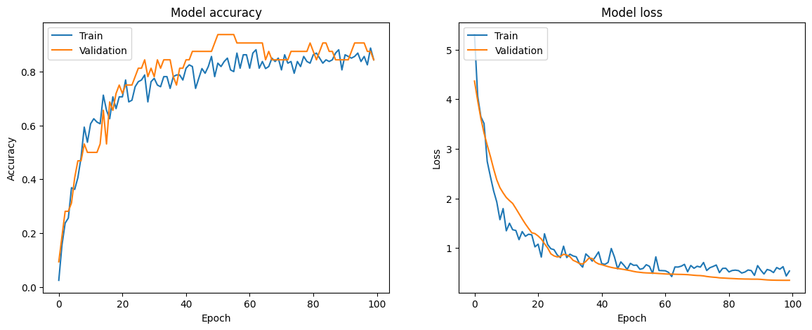
The best model showed improvement by introducing BatchNormalization before Dropout, increasing Dropout to 50%, freezing the top 10 layers, and adjusting the model checkpoint to save based on accuracy instead of validation accuracy, as validation accuracy was consistently higher during training. The training loss and accuracy curves are shown below:

The model’s training and validation accuracies both increase over time, with validation accuracy showing slight fluctuations, indicating minor overfitting. The training and validation losses both decrease and stabilize, suggesting good learning and generalization. The results are shown in the table below:
| Metric | Value |
|---|---|
| Accuracy | 0.8860 |
| F1 Score | 0.8863 |
| Precision | 0.8948 |
| Recall | 0.8860 |
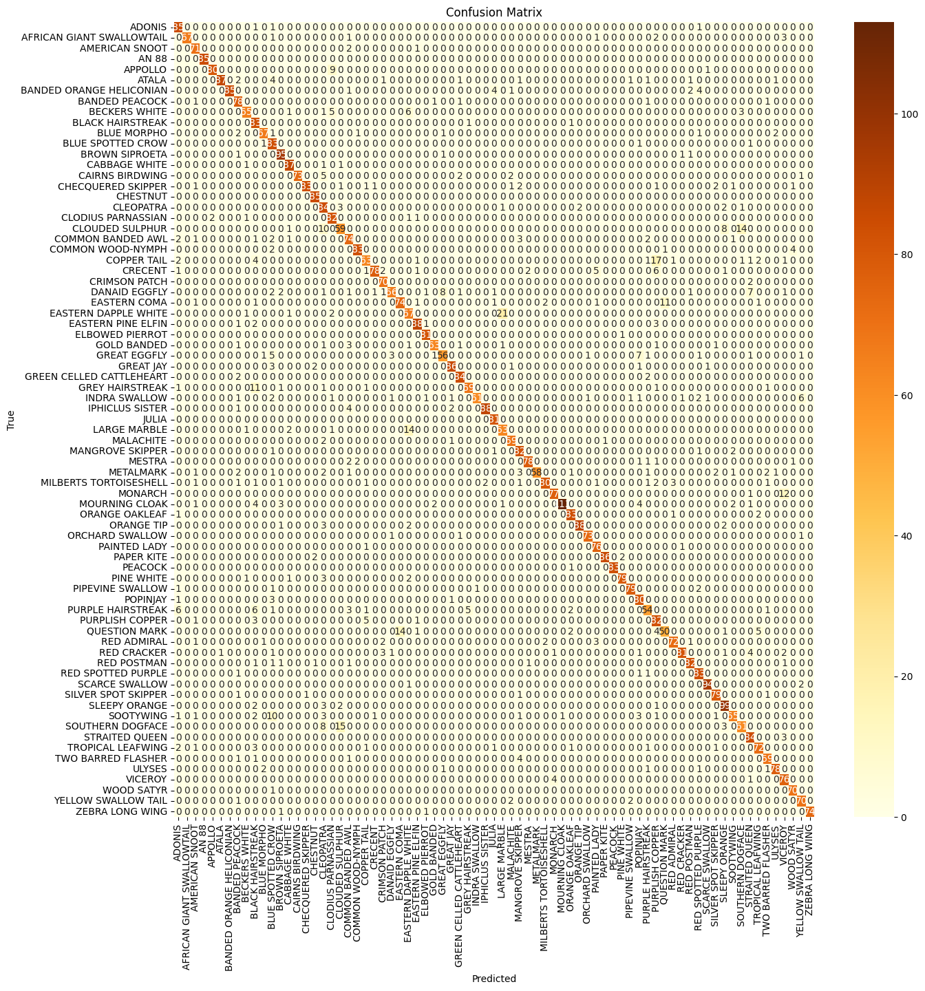
The results collectively suggest that the model is effective and reliable in its predictions, with a slight emphasis on precision. A confusion matrix was also plotted to get a better understanding of the classification performance for different classes:

The strong diagonal line shows the model correctly classifies the majority of samples for most classes, demonstrating effective learning. However, some horizontal and vertical lines of misclassifications suggest similarities between certain species. Varying diagonal intensity indicates that some classes have more samples than others, suggesting potential class imbalance. Some species have noticeable off-diagonal values, suggesting they are often misclassified with other species. Some examples are:
- “AFRICAN GIANT SWALLOWTAIL”: Misclassified as “AMERICAN SNOUT” and “AMIRAL”.
- “COMMON BANDED AWL”: Misclassified as “COMMON WOOD-NYMPH” and “CABBAGE WHITE”.
- “GREY HAIRSTREAK”: Misclassified as “INDRA SWALLOW” and “IPHICLUS SISTER”.
- “MILBERTS TORTOISESHELL”: Misclassified as “METALMARK” and “MOURNING CLOAK”.
- “RED SPOTTED PURPLE”: Misclassified as “RED RING SKIPPER” and “RED POSTMAN”.
These misclassifications suggest that these species share visual similarities or have overlapping features, leading to confusion in the model’s predictions.
Suggested Improvements
While our current model performs well, there are several ways to further enhance its accuracy and robustness:
- Increase Dataset Size: Adding more images, especially for less common species, can help the model learn better.
- Advanced Augmentation Techniques: Using more sophisticated data augmentation methods can improve the model’s generalization capabilities.
- Ensemble Methods: Combining the predictions of multiple models can yield better results than any single model.
- Further Hyperparameter Tuning: Experimenting with different hyperparameters can help find the best configuration for our model.